Why does decision tree make flat prediction?

Oh, my trained model predicts same values.
It seems wrong.

When we want to predict something that has numeric value, we sometimes use AI model.

Decision tree is one of AI model. Its process is light. So decision tree model is easy to use.

But when you use decision tree model like RandomForest or XGBoost or LightGBM, sometimes it makes flat result.

So today I will introduce about "Why does decision tree make flat prediction?".

Decision tree makes flat result

Anyway, "what is the problem ?"

If we prepare particular condition, decision tree always makes flat result.

So let's prepare the particular condition.

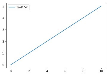
First we prepare increasing data like y=0.5x .

import matplotlib.pyplot as plt
import numpy as np
from sklearn.model_selection import train_test_split
from sklearn.ensemble import RandomForestRegressor

# dataset
x = np.linspace(0, 10, 100)
y = x * 0.5

# Set data on graph
plt.plot(x, y, label="y=0.5x")
# Set legend
plt.legend()
# Show graph
plt.show()

Once data is prepared, it shows linear graph like below.

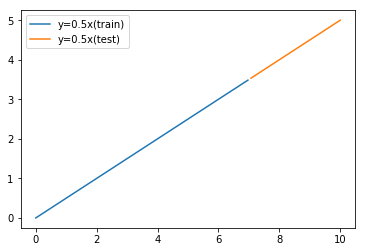
We split this data into 70% training data and remaining test data.

# split data
train_rate = 0.7
train_size = int(len(x) * train_rate)
x_train, x_test, y_train, y_test = x[0:train_size], x[train_size:len(x)], y[0:train_size], y[train_size:len(y)]

# Show graph
plt.plot(x_train, y_train, label="y=0.5x(train)")
plt.plot(x_test, y_test, label="y=0.5x(test)")
plt.legend()
plt.show()

Then linear data is separated into training data and test data.

And we train model with training data and predict with test data.
We use a kind of Decision tree model like RandomForest.

# Train and Predict
reg = RandomForestRegressor(random_state=0)
reg = reg.fit(np.array(x_train).reshape(-1,1), y_train)
y_pred = reg.predict(np.array(x_test).reshape(-1,1))

# Show graph
plt.plot(x_train, y_train, label="y=0.5x(train)")
plt.plot(x_test, y_test, label="y=0.5x(test)")
plt.plot(x_test, y_pred, label="y_pred")
plt.legend()
plt.show()

Then we get result like below.
Prediction result shows flat. It is different from actual test data.

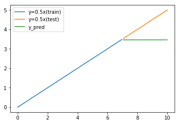
Why does this AI model fail to predict ?

In order to find the cause, let's compare with other model.

Comparing to Linear Regression

If we use Linear Regression model, it does not show flat result.

# Train and Predict
from sklearn.linear_model import LinearRegression
reg = LinearRegression()
reg = reg.fit(np.array(x_train).reshape(-1,1), y_train)
y_pred = reg.predict(np.array(x_test).reshape(-1,1))

# Show graph
plt.plot(x_train, y_train, label="y=0.5x(train)")
plt.plot(x_test, y_test, label="y=0.5x(test)")
plt.plot(x_test, y_pred, label="y_pred")
plt.legend()
plt.show()

Linear Regression model predicts like below.

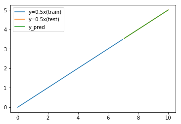
This model's prediction seems correct.

The reason why decision tree make flat prediction

The reason why decision tree make flat prediction is architecture of Decision tree.

Rule of Decision tree is below.
RandomForest and XGBoost are little bit more compricated.
But base of the architecture is same.

Important thing is "edge values are fixed by training data".
Edge values are prediction values.
They are fixed in training phase.
After training, even we input bigger data, decision route and result is always maximum one.

In last example of y=0.5x, maximum value of training data is 3.5 in case of x=7.
So trained model can't predict more than 3.5.

It means Decision tree can't predict different range from training data.

How to use decision tree with unfixed range data

So is Decision tree useless ?
No, it is not correct.

It can't predict unlimited range value.
We can use limited range value for prediction target.

As limited range value, we can use "difference".

Assume x is separated value and use difference between y of t and t-1.
So we can get stable difference for the example of y=0.5x.

import pandas as pd
df_data = pd.DataFrame()
df_data["x"] = x
df_data["y"] = y
df_data["y_diff"] = df_data["y"] - df_data["y"].shift(1)
df_data = df_data.dropna()

# split data
df_train, df_test = df_data.iloc[0:train_size], df_data.iloc[train_size:] 

# Show graph
plt.plot(df_train["x"], df_train["y_diff"], label="y=0.5x(train) diff")
plt.plot(df_test["x"], df_test["y_diff"], label="y=0.5x(test) diff")
plt.legend()
plt.show()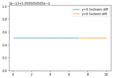

Difference range of test data is same as range of training data.
So it is suitable for prediction target.

And we add predicted difference to original y.
Then we get good prediction.

# Train and Predict difference
reg = RandomForestRegressor(random_state=0)
reg = reg.fit(np.array(df_train["x"]).reshape(-1,1), df_train["y_diff"])
y_diff_pred = reg.predict(np.array(df_test["x"]).reshape(-1,1))

# Add difference
y_pred = []
for i in range(0,len(df_test["x"])):
    if i == 0:
        y_pred.append(df_train["y"].iloc[-1] + y_diff_pred[i])
    else:
        y_pred.append(y_pred[i-1]+y_diff_pred[i])

print(y_pred)

# Show graph
plt.plot(df_train["x"], df_train["y"], label="y=0.5x(train)")
plt.plot(df_test["x"], df_test["y"], label="y=0.5x(test)")
plt.plot(df_test["x"], y_pred, label="y=0.5x(pred)")
plt.legend()
plt.show()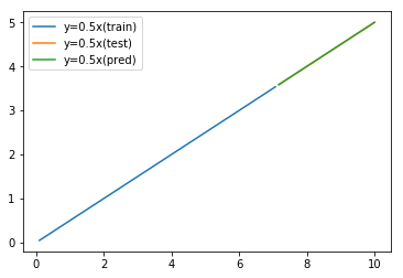

Now predicted data seems OK.

Conclusion

Today I described about "Why does decision tree make flat prediction?".

Important points are following.

Once we understand model feature, we can use it correctly.